FokkerPlanckEqExample.cpp

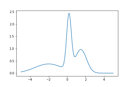
Example shows how to calculate solve diffusion equation. As the initial value we use following function:

where n(x,m,s) is density of normal distribution with mean m and standard deviation s.

We solve following equation

for and . We used Dirichlet boundary conditions, setting 0 for both ends. We used Crank-Nicolson Scheme with uniform grid.

#include <marian.hpp>
#include <cmath>

using namespace marian;

double func(double x) {
  double s1 = 0.25;
  double m1 = 0.2;
  double ret =  (1.0 / sqrt(3.14159*s1*s1))*exp(-pow(x-m1,2)/(2.0*s1*s1));
  double s2 = 0.6;
  double m2 = 1.5;  
  ret +=  (1.0 / sqrt(3.14159*s2*s2))*exp(-pow(x-m2,2)/(2.0*s2*s2));
  double s3 = 1.5;
  double m3 = -2.0;  
  ret +=  (1.0 / sqrt(3.14159*s3*s3))*exp(-pow(x-m3,2)/(2.0*s3*s3));  
  return ret;
}

int main () {
  //
  // Process
  // 
  ConvectionDiffusion process;
  process.diffusion  = 2.0;
  process.convection = 0.1;
  process.decay      = 0.2;

  //
  // Grid
  //
  int nspatial  = 100;
  int ntemporal = 400;
  UniformGridBuilder ugb;
  auto spatial_grid  = ugb.buildGrid(-5.0, 5.0, nspatial);
  auto temporal_grid = ugb.buildGrid( 0.0, 1.5, ntemporal);

  //
  // Boundary conditions
  //
  auto dbc_func = [](double)->double{return 0.0;};
  DirichletBoundaryCondition<decltype(dbc_func)> lowbc(BCSide::LOW, dbc_func);
  DirichletBoundaryCondition<decltype(dbc_func)> uppbc(BCSide::UPP, dbc_func);
  std::vector<SmartPointer<BoundaryCondition> > bcs;
  bcs.push_back(lowbc);
  bcs.push_back(uppbc);

  //
  // initial conditions
  //
  std::vector<double> f;
  for (auto x : spatial_grid) {
    f.push_back(func(x));
  }
  // Schemes
  LUSolver trisolver;
  CrankNicolsonScheme cnscheme(trisolver);
  ForwardKolmogorowEquation fokker_planck_equation(process);

  auto fdmcn = fokker_plack_equation.solveAndSave(cnscheme, f, bcs, spatial_grid, temporal_grid, "fokker_planck_equation");
}